Univariate Categorical Variable

Setup

Type library(statdata) and then, datasets in the statdata package are avaiable.

library(tidyverse)
#> ── Attaching packages ─────────────────────────────────────── tidyverse 1.3.1 ──
#> ✓ ggplot2 3.3.5     ✓ purrr   0.3.4
#> ✓ tibble  3.1.4     ✓ dplyr   1.0.7
#> ✓ tidyr   1.1.3     ✓ stringr 1.4.0
#> ✓ readr   2.0.1     ✓ forcats 0.5.1
#> ── Conflicts ────────────────────────────────────────── tidyverse_conflicts() ──
#> x dplyr::filter() masks stats::filter()
#> x dplyr::lag()    masks stats::lag()
library(statdata)

Load Sample Dataset

gender dataset contains male and female row-by-row values.

data("gender")
gender <- gender %>% 
  set_names("gender")

gender
#> # A tibble: 10 × 1
#>    gender
#>    <chr> 
#>  1 남    
#>  2 여    
#>  3 남    
#>  4 여    
#>  5 남    
#>  6 남    
#>  7 남    
#>  8 여    
#>  9 여    
#> 10 남

Basic Analysis

The univariate categorical variable can be summarized through counting.

gender %>%
  count(gender)
#> # A tibble: 2 × 2
#>   gender     n
#>   <chr>  <int>
#> 1 남         6
#> 2 여         4

Visualization

We can visualize the univariate categorical variable with barplot or pie chart.

par(family = "NanumGothic")

gender_count <- gender %>%
  count(gender)

barplot(n ~ gender, data = gender_count)

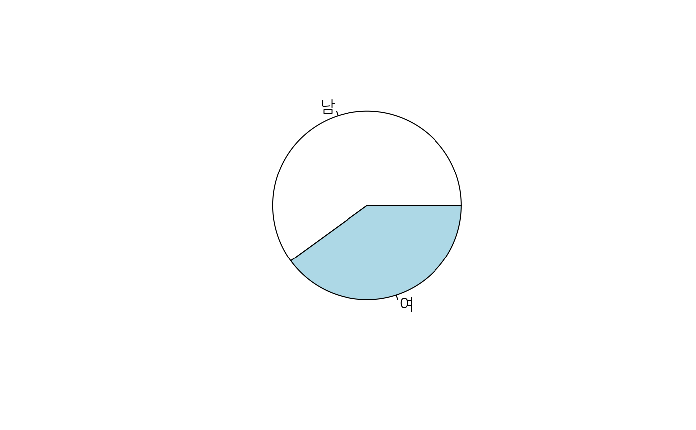
The pie chart plot is also possible.

par(family = "NanumGothic")

gender_vector <- gender_count %>% 
  pull(n)

names(gender_vector) <- gender_count$gender

pie(gender_vector)