Univariate Continous Variable

Setup

Type library(statdata) and then, datasets in the statdata package are avaiable.

library(tidyverse)
#> ── Attaching packages ─────────────────────────────────────── tidyverse 1.3.1 ──
#> ✓ ggplot2 3.3.5     ✓ purrr   0.3.4
#> ✓ tibble  3.1.4     ✓ dplyr   1.0.7
#> ✓ tidyr   1.1.3     ✓ stringr 1.4.0
#> ✓ readr   2.0.1     ✓ forcats 0.5.1
#> ── Conflicts ────────────────────────────────────────── tidyverse_conflicts() ──
#> x dplyr::filter() masks stats::filter()
#> x dplyr::lag()    masks stats::lag()
library(statdata)

Load Sample Dataset

kicks_num dataset contains number of success in the traditional Korean game, Jegichagi.

data("kicks_num")
kicks_num <- kicks_num %>% 
  set_names('count')

kicks_num
#> # A tibble: 30 × 1
#>    count
#>    <dbl>
#>  1    32
#>  2    46
#>  3    54
#>  4    27
#>  5    16
#>  6    52
#>  7    18
#>  8    45
#>  9    47
#> 10    36
#> # … with 20 more rows

Basic Analysis

skimr package contains skim() function, which is an improved version of summary function. This one line command spits out all the descriptive statstics needed to understand the continuous variable.

skimr::skim(kicks_num)

Data summary

Name	kicks_num
Number of rows	30
Number of columns	1
_______________________
Column type frequency:
numeric	1
________________________
Group variables	None

Variable type: numeric

skim_variable	n_missing	complete_rate	mean	sd	p0	p25	p50	p75	p100	hist
count	0	1	33.9	14.44	12	25	30	46.75	59	▇▇▃▆▅

Visualization

We can visualize the univariate continouse variable with histogram or stem-and-leaf plot. There are various ways to visualize histogram, but the simplest way is to use hist().

hist(kicks_num$count)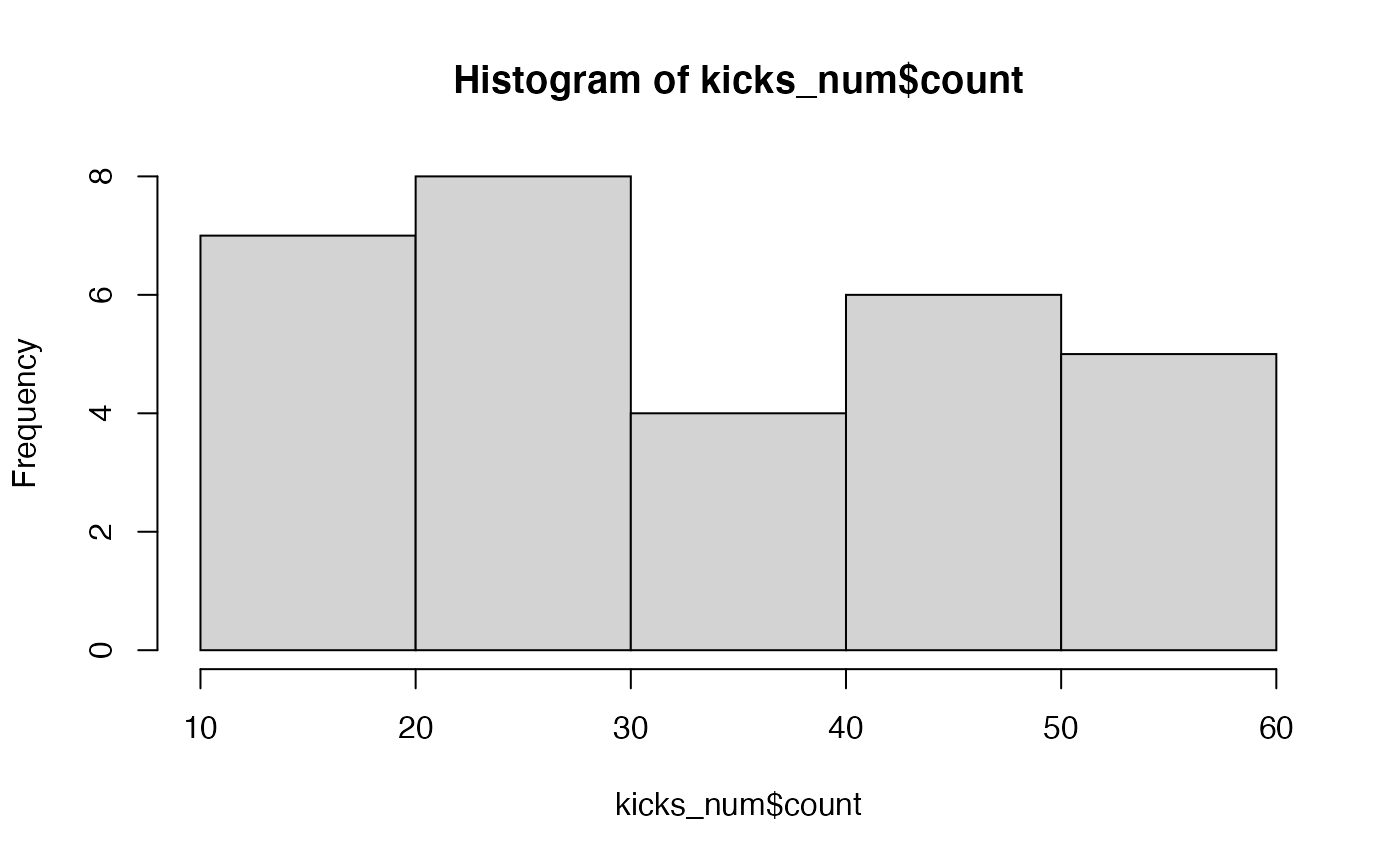

The stem-and-leaf plot is also possible.

stem(kicks_num$count)
#> 
#>   The decimal point is 1 digit(s) to the right of the |
#> 
#>   1 | 24
#>   1 | 67889
#>   2 | 
#>   2 | 55567778
#>   3 | 23
#>   3 | 66
#>   4 | 4
#>   4 | 56778
#>   5 | 24
#>   5 | 599